

이번 사이드 프로젝트는 Santander Customer Satisfaction 데이터로 고객 불만족(타겟=1)을 예측하는 이진 분류(Binary Classification) 문제입니다.
데이터의 특징은 극심한 클래스 불균형이며, 실제 분포는 다음과 같습니다.
- TARGET=0(만족): 73,012건
- TARGET=1(불만족): 3,008건
- 불만족 비율: 0.04(약 4%)
즉, “대부분이 만족(0)”인 데이터에서 “소수의 불만족(1)”을 얼마나 잘 찾아내느냐가 핵심이며, 그래서 평가 지표를 Accuracy가 아닌 ROC-AUC로 두는 흐름이 매우 합리적입니다.
1. 데이터 전처리
1-1) 데이터 로딩 및 기본 확인
import numpy as np
import pandas as pd
import matplotlib.pyplot as plt
import warnings
warnings.filterwarnings('ignore')

# (1) 데이터 로딩
cust_df = pd.read_csv('./customer/santander-customer-satisfaction/train_santander.csv')

# (2) shape 확인: (행 수, 열 수)
print(f"shape : {cust_df.shape}")

# (3) 상위 3개 샘플 확인 (데이터 감 잡기)
display(cust_df.head(3))

# (4) 컬럼 타입/결측치/메모리 사용량 확인
cust_df.info()

1-2) 타겟 분포 확인 (불균형 데이터)
# TARGET=1(불만족) 개수
unsatisfied_cnt = cust_df[cust_df['TARGET'] == 1].TARGET.count()

# 전체 데이터 개수
total_cnt = cust_df.TARGET.count()

# 불만족 비율(=양성 클래스 비율) 계산
print(f'Unsatisfied Rate : {round((unsatisfied_cnt / total_cnt), 2)}')

# 결과(사용자 실행 로그):
# Unsatisfied Rate : 0.04- 위 결과에서 확인되듯 양성 클래스(불만족=1)가 4% 수준입니다.
- 이런 경우 단순 정확도는 왜곡될 수 있어, 이후 평가를 ROC-AUC로 진행합니다.
1-3) 이상치/불필요 컬럼 처리
사용자 분석대로 var3에서 -999999는 정상적인 값이라 보기 어렵고, 보통 “결측/이상값 마킹”으로 쓰이는 경우가 많습니다. 따라서 이를 대표값(여기서는 2)으로 치환합니다.
# (1) describe()로 전반적 통계 확인
cust_df.describe()

# (2) var3의 값 분포 확인: -999999가 다수 존재하면 이상치/결측 마킹일 가능성 큼
cust_df['var3'].value_counts()

# (3) var3의 -999999를 2로 대체
# - 사용자 판단: -999999는 이상치로 보고 대표값 2로 치환
cust_df['var3'].replace(-999999, 2, inplace=True)

# (4) ID 컬럼 제거
# - 식별자(ID)는 모델 학습에 의미 있는 신호가 아니라서 보통 제거
cust_df.drop('ID', axis=1, inplace=True)
1-4) 피처/레이블 분리
# (1) 피처(X): TARGET 제외 나머지
X_features = cust_df.iloc[:, :-1]

# (2) 레이블(y): TARGET
y_labels = cust_df.iloc[:, -1]

print(f'feature shape : {X_features.shape}')
print(f'label shape : {y_labels.shape}')

# 사용자 로그 기준:
# feature shape : (76020, 369)
# label shape   : (76020,)
2. 데이터 셋 분리 (Train/Test + Train/Validation)
이 프로젝트는 **조기 종료(Early Stopping)**를 쓰기 때문에, 일반 Train/Test 외에도 Train 내부를 Train/Validation으로 한 번 더 분리합니다.
from sklearn.model_selection import train_test_split

# =========================================================
# 2-1) Train/Test 분리 (80% / 20%)
# - stratify=y_labels: 불균형 클래스 비율을 Train/Test에서 동일하게 유지
# =========================================================
X_train, X_test, y_train, y_test = train_test_split(
    X_features,
    y_labels,
    test_size=0.2,
    random_state=0,
    stratify=y_labels
)

print(f'학습셋 : {X_train.shape}')
print(f'테스트셋 : {X_test.shape}')

# 사용자 실행 로그:
# 학습셋 : (60816, 369)
# 테스트셋 : (15204, 369)

# =========================================================
# 2-2) Train을 다시 Train/Validation으로 분리 (70% / 30%)
# - Early Stopping 성능 평가용 Validation 세트
# =========================================================
X_tr, X_val, y_tr, y_val = train_test_split(
    X_train,
    y_train,
    test_size=0.3,
    random_state=0,
    stratify=y_train
)

print(f'학습셋(분리 후) : {X_tr.shape}')
print(f'검증셋 : {X_val.shape}')

# 사용자 실행 로그:
# 학습셋(분리 후) : (42571, 369)
# 검증셋 : (18245, 369)
3. XGBoost 모델 학습 및 HyperOpt 튜닝
3-1) 1차 시도: 기본 XGBoost + Early Stopping
from xgboost import XGBClassifier
from sklearn.metrics import roc_auc_score

# (1) 기본 모델 구성
# - n_estimators=500: 트리 500개까지 학습 가능
# - learning_rate=0.05: 학습률(작을수록 천천히, 보통 n_estimators와 함께 조정)
# - random_state=156: 재현성(항상 같은 결과)
xgb_clf = XGBClassifier(
    n_estimators=500,
    learning_rate=0.05,
    random_state=156
)

# (2) Early Stopping을 위한 eval_set 구성
# - (X_tr, y_tr): 학습 성능 추적용
# - (X_val, y_val): 검증 성능 추적용(중요: early stopping 기준)
eval_set = [(X_tr, y_tr), (X_val, y_val)]

# (3) 학습 수행
# - eval_metric='auc': 검증 성능을 ROC-AUC로 측정하며 개선 여부 판단
# - early_stopping_rounds=100: 100번 연속으로 auc 개선 없으면 중단
xgb_clf.fit(
    X_tr,
    y_tr,
    early_stopping_rounds=100,
    eval_metric='auc',
    eval_set=eval_set
)

# (4) 테스트 데이터에서 확률 예측(ROC-AUC는 확률 기반 지표)
pred_proba = xgb_clf.predict_proba(X_test)[:, 1]

# (5) ROC-AUC 평가
xgb_roc_score = roc_auc_score(y_test, pred_proba)
print(f'ROC AUC : {xgb_roc_score}')

# 사용자 실행 로그:
# ROC AUC : 0.8233085191533859
3-2) 2차 시도: HyperOpt(TPE) 기반 베이지안 튜닝
(1) Search Space 정의
from hyperopt import hp

# HyperOpt는 "범위"를 주면 그 안에서 값을 뽑아 시도합니다.
# quniform은 간격(step)이 있는 분포(하지만 결과가 float이므로 int 변환 필요)
xgb_search_space = {
    'max_depth': hp.quniform('max_depth', 5, 20, 1),
    'min_child_weight': hp.quniform('min_child_weight', 1, 6, 1),
    'colsample_bytree': hp.uniform('colsample_bytree', 0.5, 0.95),
    'learning_rate': hp.uniform('learning_rate', 0.01, 0.2)
}
(2) Objective Function 정의: “ROC-AUC 평균을 최대화”
여기서 중요한 흐름은 다음과 같습니다.
- HyperOpt는 기본적으로 loss를 최소화
- 우리는 ROC-AUC를 최대화하고 싶음
- 따라서 loss = -roc_auc_mean 형태로 반환
또한 사용자는 KFold(n_splits=3)로 직접 CV를 구현했습니다.
(불균형 데이터라면 StratifiedKFold가 더 일반적이지만, 사용 코드 흐름을 유지하되 주석에서 관점을 보완합니다.)
from sklearn.model_selection import KFold
from sklearn.metrics import roc_auc_score
from xgboost import XGBClassifier

def objective_func(search_space):
    """
    목적 함수(Objective Function)
    - 입력: HyperOpt가 샘플링한 하이퍼파라미터 조합(search_space)
    - 처리: 3-Fold 교차검증으로 ROC-AUC 평균 계산
    - 출력: HyperOpt가 최소화할 loss 반환 (loss = -mean_auc)
    """

    # (1) HyperOpt에서 넘어오는 값은 float 형태 → 정수형 파라미터는 int로 변환
    xgb_clf = XGBClassifier(
        n_estimators=100,  # 튜닝 단계에서는 속도 절약을 위해 100으로 축소(사용자 의도)
        max_depth=int(search_space['max_depth']),
        min_child_weight=int(search_space['min_child_weight']),
        colsample_bytree=search_space['colsample_bytree'],
        learning_rate=search_space['learning_rate'],
        eval_metric='auc',
        random_state=156,
        n_jobs=-1
    )

    roc_auc_list = []

    # (2) KFold로 Train 데이터를 3개 폴드로 분할
    # - 불균형 문제가 크면 StratifiedKFold가 더 안정적일 수 있음
    kf = KFold(n_splits=3)

    for tr_index, val_index in kf.split(X_train):
        # (3) fold별 학습/검증 데이터 구성
        X_tr_fold, y_tr_fold = X_train.iloc[tr_index], y_train.iloc[tr_index]
        X_val_fold, y_val_fold = X_train.iloc[val_index], y_train.iloc[val_index]

        # (4) fold 내부에서도 early stopping 적용
        # - 30번 동안 AUC 개선 없으면 학습 중지 → 시간 절약 + 과적합 방지
        xgb_clf.fit(
            X_tr_fold,
            y_tr_fold,
            early_stopping_rounds=30,
            eval_metric='auc',
            eval_set=[(X_tr_fold, y_tr_fold), (X_val_fold, y_val_fold)],
            verbose=False
        )

        # (5) 검증 fold에서 ROC-AUC 계산
        val_pred_proba = xgb_clf.predict_proba(X_val_fold)[:, 1]
        score = roc_auc_score(y_val_fold, val_pred_proba)
        roc_auc_list.append(score)

    # (6) 3개 fold ROC-AUC 평균
    mean_auc = np.mean(roc_auc_list)

    # (7) HyperOpt는 loss 최소화 → AUC 최대화를 위해 -1 곱해서 반환
    return -1 * mean_auc
(3) fmin 실행: 50회 탐색
from hyperopt import fmin, tpe, Trials

trials = Trials()

best = fmin(
    fn=objective_func,
    space=xgb_search_space,
    algo=tpe.suggest,
    max_evals=50,
    trials=trials,
    rstate=np.random.default_rng(seed=30)
)

print(f'Best 하이퍼 파라미터 : {best}')

# 사용자 실행 로그:
# Best 하이퍼 파라미터 : {
#   'colsample_bytree': 0.7958795930205148,
#   'learning_rate': 0.11599863372320877,
#   'max_depth': 5.0,
#   'min_child_weight': 4.0
# }
(4) Best 파라미터로 “실제 학습(n_estimators=500)” 후 테스트 평가
튜닝 단계에서는 n_estimators=100으로 속도를 줄였고,
최종 학습에서는 다시 n_estimators=500으로 올려 성능을 확인하는 흐름이 깔끔합니다.
from sklearn.metrics import roc_auc_score
from xgboost import XGBClassifier

# (1) HyperOpt가 찾아준 best 파라미터를 반영
xgb_clf = XGBClassifier(
    n_estimators=500,
    learning_rate=round(best['learning_rate'], 5),
    max_depth=int(best['max_depth']),
    min_child_weight=int(best['min_child_weight']),
    colsample_bytree=round(best['colsample_bytree'], 5),
    eval_metric='auc',
    random_state=156,
    n_jobs=-1
)

evals = [(X_tr, y_tr), (X_val, y_val)]

# (2) early stopping 적용 후 학습
xgb_clf.fit(
    X_tr,
    y_tr,
    early_stopping_rounds=100,
    eval_metric='auc',
    eval_set=evals
)

# (3) 테스트 ROC-AUC 평가
pred_proba = xgb_clf.predict_proba(X_test)[:, 1]
xgb_roc_score = roc_auc_score(y_test, pred_proba)
print(f'ROC AUC : {xgb_roc_score}')

# 사용자 실행 로그:
# ROC AUC : 0.825153599311249- 1차(기본): 0.8233085
- 2차(HyperOpt): 0.8251536
개선 폭이 크진 않지만, 조합 탐색을 “체계적으로” 수행해 개선을 확인했다는 점이 프로젝트 관점에서 의미가 있습니다.
(5) 피처 중요도 시각화
from xgboost import plot_importance
import matplotlib.pyplot as plt

fig, ax = plt.subplots(1, 1, figsize=(10, 8))

plot_importance(
    xgb_clf,
    ax=ax,
    max_num_features=20,
    height=0.4
)

plt.show()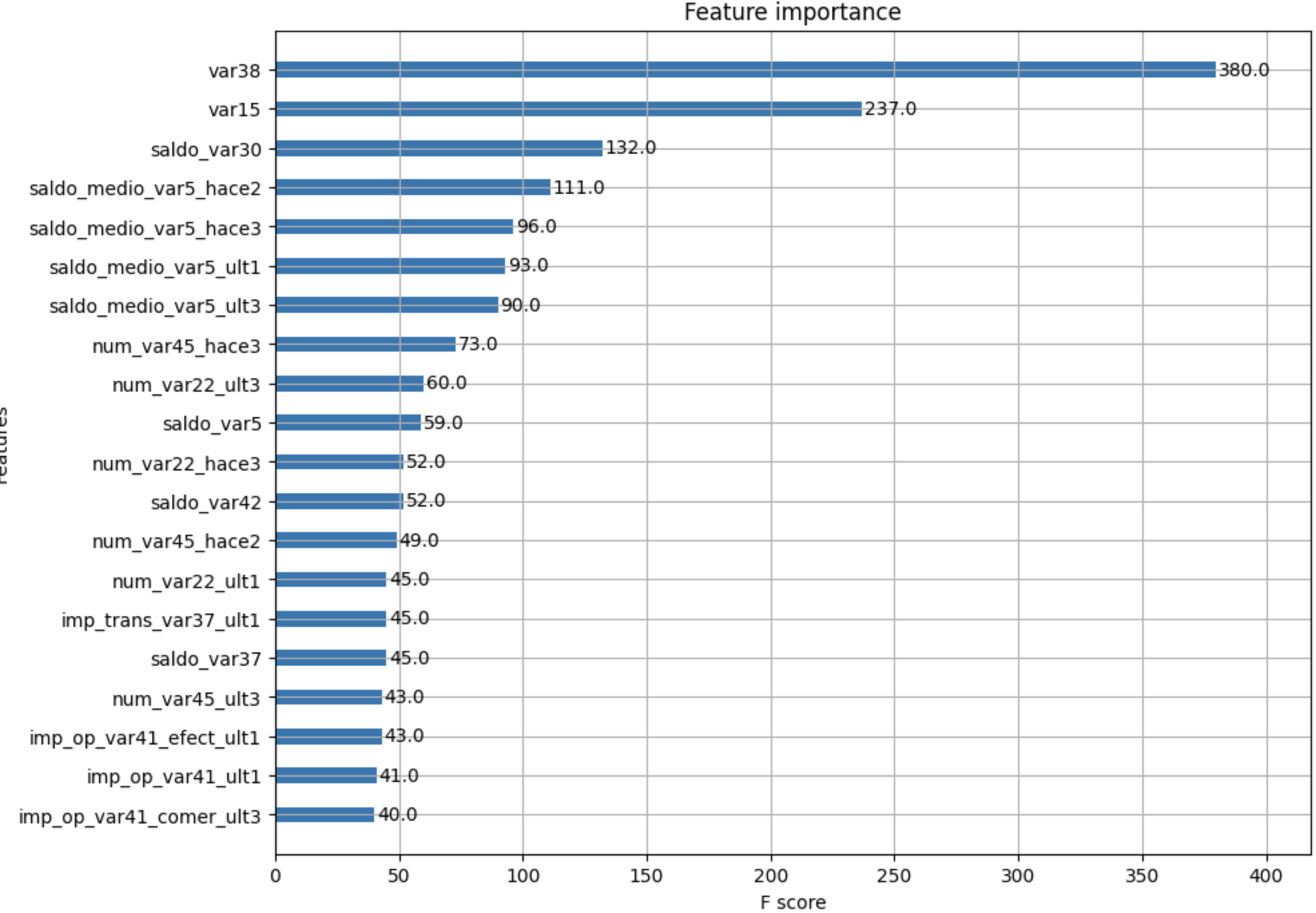
4. LightGBM 모델 학습 및 HyperOpt 튜닝
사용자 코멘트처럼 LightGBM은 트리 구조에서 max_depth도 중요하지만, 실무에서는 **num_leaves(리프 개수)**가 핵심 파라미터로 자주 언급됩니다. (리프 기반 성장 특성 때문에)
4-1) 튜닝 전 기본 LightGBM
from lightgbm import LGBMClassifier, early_stopping
from sklearn.metrics import roc_auc_score

# (1) 기본 모델
lgbm_clf = LGBMClassifier(
    n_estimators=500,
    random_state=156
)

eval_set = [(X_tr, y_tr), (X_val, y_val)]

# (2) 학습 (AUC 기준 early stopping)
lgbm_clf.fit(
    X_tr,
    y_tr,
    eval_set=eval_set,
    eval_metric='auc',
    callbacks=[early_stopping(stopping_rounds=100)]
)

# (3) 테스트 ROC-AUC
pred_proba = lgbm_clf.predict_proba(X_test)[:, 1]
lgbm_roc_score = roc_auc_score(y_test, pred_proba)
print(f"ROC AUC : {lgbm_roc_score}")

# 사용자 실행 로그:
# ROC AUC : 0.8213213522381906
4-2) HyperOpt로 LightGBM 튜닝
(1) Search Space
from hyperopt import hp

lgbm_search_space = {
    'num_leaves': hp.quniform('num_leaves', 32, 64, 1),
    'max_depth': hp.quniform('max_depth', 100, 160, 1),
    'min_child_samples': hp.quniform('min_child_samples', 60, 100, 1),
    'subsample': hp.uniform('subsample', 0.7, 1.0),
    'learning_rate': hp.uniform('learning_rate', 0.01, 0.2)
}
(2) Objective Function
from sklearn.model_selection import KFold
from sklearn.metrics import roc_auc_score
from lightgbm import LGBMClassifier, early_stopping

def objective_func(search_space):
    """
    LightGBM 목적 함수
    - 3-Fold CV로 ROC-AUC 평균을 계산
    - HyperOpt가 최소화하도록 loss=-mean_auc 반환
    """

    lgbm_clf = LGBMClassifier(
        n_estimators=100,  # 튜닝 속도 절약
        num_leaves=int(search_space['num_leaves']),
        max_depth=int(search_space['max_depth']),
        min_child_samples=int(search_space['min_child_samples']),
        subsample=search_space['subsample'],
        learning_rate=search_space['learning_rate'],
        random_state=156
    )

    roc_auc_list = []
    kf = KFold(n_splits=3)

    for tr_index, val_index in kf.split(X_train):
        X_tr_fold, y_tr_fold = X_train.iloc[tr_index], y_train.iloc[tr_index]
        X_val_fold, y_val_fold = X_train.iloc[val_index], y_train.iloc[val_index]

        eval_set = [(X_tr_fold, y_tr_fold), (X_val_fold, y_val_fold)]

        lgbm_clf.fit(
            X_tr_fold,
            y_tr_fold,
            eval_metric='auc',
            eval_set=eval_set,
            callbacks=[early_stopping(30)],
            verbose=False
        )

        val_pred_proba = lgbm_clf.predict_proba(X_val_fold)[:, 1]
        score = roc_auc_score(y_val_fold, val_pred_proba)
        roc_auc_list.append(score)

    return -1 * np.mean(roc_auc_list)
(3) fmin 실행 및 Best 파라미터로 최종 학습/평가
from hyperopt import fmin, tpe, Trials

trials = Trials()

best = fmin(
    fn=objective_func,
    space=lgbm_search_space,
    algo=tpe.suggest,
    max_evals=50,
    trials=trials,
    rstate=np.random.default_rng(seed=30)
)

print(f'best 파라미터 : {best}')

# 사용자 실행 로그:
# best 파라미터 : {
#   'learning_rate': 0.03551933341235436,
#   'max_depth': 160.0,
#   'min_child_samples': 61.0,
#   'num_leaves': 32.0,
#   'subsample': 0.8555931419795748
# }

# 최종 모델(트리 500개)로 재학습 후 테스트 ROC-AUC 확인
lgbm_clf = LGBMClassifier(
    n_estimators=500,
    num_leaves=int(best['num_leaves']),
    max_depth=int(best['max_depth']),
    min_child_samples=int(best['min_child_samples']),
    subsample=round(best['subsample'], 5),
    learning_rate=round(best['learning_rate'], 5),
    random_state=156
)

eval_set = [(X_tr, y_tr), (X_val, y_val)]

lgbm_clf.fit(
    X_tr,
    y_tr,
    eval_metric='auc',
    eval_set=eval_set,
    callbacks=[early_stopping(30)]
)

lgbm_roc_score = roc_auc_score(y_test, lgbm_clf.predict_proba(X_test)[:, 1])
print(f'roc score : {lgbm_roc_score}')

# 사용자 실행 로그 일부:
# [88] training's auc: 0.895356 ... valid_1's auc: 0.844823 ...
# roc score : 0.8239600819256998
- 기본 LightGBM: 0.8213213
- HyperOpt LightGBM: 0.8239601
정리: 이번 프로젝트에서 얻은 결론
- **데이터가 불균형(불만족 4%)**이므로, 정확도보다 ROC-AUC가 더 적절한 평가 지표입니다.
- 기본 XGBoost가 이미 성능이 좋았고, HyperOpt 튜닝으로 **AUC가 소폭 개선(0.8233 → 0.8251)**되었습니다.
- LightGBM도 HyperOpt 튜닝으로 **AUC가 개선(0.8213 → 0.8240)**되었습니다.
- 튜닝에서 하이퍼파라미터를 너무 많이 잡으면 탐색이 어려워지므로, 사용자가 정리한 것처럼 6~9개 내외로 제한하는 접근이 실무적으로 합리적입니다.
'Programming' 카테고리의 다른 글
| Credit Card Fraud Detection 1편 : Feature Engineering과 Baseline 모델 성능 분석 (0) | 2025.12.26 |
|---|---|
| IQR과 SMOTE 이해하기 (1) | 2025.12.26 |
| (Bayesian Optimization 2편) HyperOpt로 XGBoost 하이퍼파라미터 튜닝 실습 (0) | 2025.12.22 |
| (Bayesian Optimization 1편) GridSearch · RandomSearch · Bayesian Optimization 개념 완전 정리 (1) | 2025.12.22 |
| 앙상블 학습 3편: 부스팅(Boosting) · GBM · XGBoost · LightGBM 완전 정리 (0) | 2025.12.20 |